1. Background
A produced oil is a mixture of water, oil and solids in oil production facilities. The produced oil is commonly stabilized by natural surface active agents and requires intensive chemical and physical treatments to separate water and solids from the oil. Knowing water distribution, interfacial levels (or phase boundaries) and interfacial thicknesses in any process vessel are crucial to both operation engineers and R&D scientists. Water and basic sediment (BS&W) content in oil must be well controlled to be less than 0.5% for acceptance of downstream pipeline transportation. Enhanced oil recovery technologies are extensively used everywhere, various chemicals are added to improve oil recovery and added chemicals help oil to liberate from the surface of oil sands and then form a dispersion either in the form of oil-in-water (O/W) or water-in-oil (W/O) emulsion, which adversely impacts subsequent treatments of produced oils.
Water distribution analysis and phase boundary identification are lab-intensive work. Phase boundary visual identification is very difficult for heavy oils due to their dark, viscous and sticky nature. However, it is a must in both engineering and operation stages to figure out the best types of chemicals, dosages, chemical working temperature and adding procedure as well as chemical adding location in a line of production and separation vessels, e.g. well heads, well lines, gas and free water knock out vessels, oil/water separation vessels and oil purification vessels. Phase boundaries or interfacial levels can be used to evaluate how much clean oil, emulsion, rag layer and aqueous phases are present in a process vessel. Interfacial thicknesses provide additional information for evaluating the effectiveness of added chemicals. Water analysis is also important in quality assurance in various downstream oil products (such as fuels and lubricants) and other industry products (such as paints and polymers).
To do water analysis in a lab, firstly, oil samples are taken in bulks at fields and sub-sampled in the lab in multiple testing bottles for water distribution and phase boundary identification; secondly, chemicals are added to the testing samples and mixed thoroughly on a shaker followed by keeping the samples in a thermostat or water bath at a desired temperature for a certain duration to allow phase separation; thirdly, a few small amounts of samples are withdrawn using a syringe from each sample bottle at different vertical levels for subsequent water or BS&W analysis; finally, the water or BS&W analysis can be done using one or in a combination of the three methods: centrifuge [such as ASTM D1796-11(2016), ASTM D4007-11(2016), ASTM D2709-16], distillation (such as ASTM D95 and ASTM D4006) and Karl Fischer titration [such as ASTM D4928-12(2018), ASTM D6304-16, ASTM D4017, ASTM D6869-17, ASTM E203-16, ASTM E1064-16].
Both centrifuge method and distillation method involve the use of one of toxic and flammable diluents: such as toluene, xylene, petroleum naphtha, petroleum spirit and other petroleum distillates having a boiling point range of 90-210 ℃. There is a strong health and environmental safety concern about using such toxic and flammable diluents. The Karl Fischer titration method also involves the use of toxic Karl Fisher reagents, which consist of an alcohol (ethanol or diethylene glycol monoethyl ether ), a base (imidazole or pyridine), sulfur dioxide (SO2) and iodine (I2). All three methods can only provide water or BS&W content at one or a few vertical levels of a testing sample in a bottle. The centrifuge method requires at least 5 ml sample, taking 3 samples from 3 vertical levels of a 150-200 ml bottle is operable, however, taking 5 samples is extremely difficult, meaning that it is very limited for water distribution and phase boundary identification. The distillation method requires a large volume of sample, e.g. 25 ml for water content less than 10% by volume, and 200 ml for water content less than 1% by volume, meaning that it is not suitable for water distribution analysis of a sample in a 150-200 ml sample bottle. Only the Karl Fisher titration method is suitable for water distribution analysis and phase boundary identification as it just requires a small amount of sample.
Hence, it is highly desirable to have an apparatus and method for measuring water distribution, surface/interfacial levels and thicknesses of a multiphase dispersion continuously. Multi-channel scanning water analyzer (MCSWA) is such a new tool for R&D scientists, design and operational engineers to do chemical screening efficiently. MCSWA is a proprietary technology developed by M & T Instruments Ltd. and is in patent pending status.
2. Validation
To validate the instrument, four of the same used-engine oil samples were used to check its performance. Fig.1 shows a scanned result. The capacitance, C(x), is capacitance change relative to the front baseline reference; the derivative, C'(x) = dC(x)/dx , is derived from C(x) numerically; and x is bottle mark in ml. As shown in Fig. 1, four capacitance curves, C(x), had an abrupt increase at the touching of the oil sample surface when the sensors moved from the air into the oil samples, and then kept increasing proportionally to its scanned volume of the oil samples. The straight lines, C(x), in parallel for the period of scanning the oil samples, indicate that the 4 channels are consistent with each other. The derivative curves, C'(x), showing flat lines also indicate that the 4 channels are consistent with each other.
The capacitance curves, C(x), should show different slopes, and the derivative, C'(x), should move up and down accordingly if the 4 oil samples contain different water contents or have a water gradient at different bottle marks.

3. Multi-channel scan
To test the 4 channels in a full range approximately a 1:1 water-to-oil volume ratio was used. Firstly, four oil samples were prepared by adding pre-calculated amount of water to 75 ml used-engine oil in 4 bottles separately so that the oil samples contain 0.00g, 2.50g, 5.00g and 10.00g water per 100 ml oil respectively and then the mixtures were well mixed on a shaker to form emulsions; secondly, the resultant oil samples were added slowly to the top of 75 ml water with extreme care to minimize mixing; Thirdly, the sample bottles having the emulsion on top and the aqueous at the bottom were kept in the heating cells for phase separation; lastly, a full range scan was conducted at different settling times: 2 hours, 6 hours and 18 hours, respectively. Fig. 2 below is one of the scanned results.
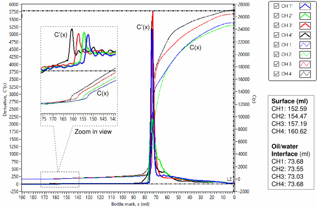
There are two significant variations in both capacitance and derivative at the top oil surface and the middle oil/water interface. The variation at the top oil surface is very small compared with it at the middle oil/water interface because most hydrocarbons have their dielectric constants in a range of 1.8-2.5, while water has a dielectric constant of 80. The curve’s variations at the top oil surface can be clearly observed in the embedded zoom-in view. The top oil surface and the middle oil/water interface levels can be automatically determined accurately using data processing, Both of them are also listed in FIG. 2.
The most important part is the water profiles in the top organic phases. Details are shown in Figs 3, 4 and 5 for settling times of 2 hours, 6 hours and 18 hours, respectively. It can be seen that capacitance curves, C(x), are linear at the top part and nonlinear at the bottom part of the organic phases. For the linear parts of the curves, it is believed that water is evenly distributed, which is similar to the situation shown in Fig.1 for the oil samples with no added water. Actually, CH1 in Fig.2 represents the oil sample with no added water. For the nonlinear parts of the curves, it is believed that water is not evenly distributed. The gradient (or the derivative) of a curve at a given bottle mark is a reflection of water distribution at the bottle mark. It is straightforward that the greater the slope of a curve of capacitance the higher the water content in the oil. Hence, a ranking in water content in oil samples can be made by direct visual comparison of the scanned curves. The ranking visually in water content in the top parts of the organic phases is CH4 > CH3 > CH2 > CH1. More precisely, the slopes of the curve’s linear parts (from bottle mark 110 to 150 ml) can be derived via data processing and the consistent result is summarized in Fig. 6.


Comparing Figs. 3, 4 and 5, it can be observed that, increasing the settling time, capacitance curves were getting closer and closer to the curve of CH1, which was for the oil sample with no added water, indicating dewatering was in progress. In addition, the slopes of the linear parts of the curves were also getting closer and closer to parallel to each other, which is confirmed by the numbers summarized in Fig. 6. In other wards, with increasing the settling time, the water contents were getting closer to each other.
The derivative curves, C'(x), can not only be used to determine the top surface and the middle interface levels but also to determine the starting point and the ending point of the linear part by looking at the flat part of the curves, e.g. the period from bottle mark 110 ml to 150 ml can be safely considered as flat in C'(x) curves and linear in C(x) curves.
4. Scanning multi-phase to measure water distribution, interfacial levels and thicknesses
Fig. 7 is an example of scanned curves of capacitance Ca(x) and Cb(x), and their derivative Ca'(x) and Cb'(x) for 2 channels (for sample bottles A and B). Fig. 8 is a zoom-in view of Fig. 7 for detailed view of the low value parts. There are 4 phases in bottle A, their interfaces are labelled as A1, A2, A3 and A4 in the inserted photo, where the 4 phases are a clean oil phase between A1 and A2, an emulsion phase between A2 and A3, a rag layer phase between A3 and A4 and an aqueous phase at the bottom. There are only 2 phases in bottle B, their interfaces are labelled as B1 and B2, where the 2 phases are a clean oil phase at the top and an emulsion phase at the bottom.
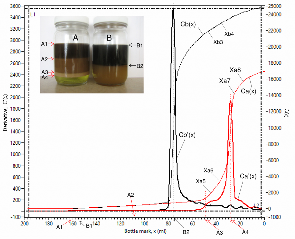
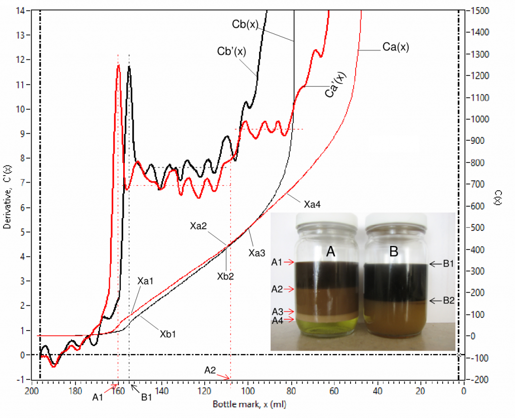
The derivative C'(x) is advantageous in interfacial level identification as it shows spikes at every interface, denoted using volume in ml starting from the bottom of a bottle, e.g. A1 (160.00 ml), A2 (107.90 ml), A3(48.03 ml) and A4 (28.18 ml) for sample bottle A; B1 (154.70 ml) and B2 (75.89 ml) for sample bottle B. The coordination values [x, C'(x) ] are shown simultaneously on the computer screen when the vertical cursor lines (L1 and L2) are dragged and moved. The water contents in different phases can be obtained from capacitance curve using linear fittings for specified data ranges that show linear trends, such as (Xa1 – Xa2), (Xa3 – Xa4), (Xa5 – Xa6) and (Xa7 – Xa8) for Ca(x) and (Xb1 – Xb2) and (Xb3 – Xb4) for Cb(x) . Water content by volume percent, W(x) , is proportional to the slope, S(x) , of a linear-fitted line,

where K is a capacitive coefficient of a testing sample. So, one can have Wa(x) = KaSa(x), Wb(x) = KbSb(x), etc. where Ka and Kb are the capacitive coefficients of samples A and B respectively, which can be obtained using a calibration curve. A summary of processed data is shown below in Table 1.
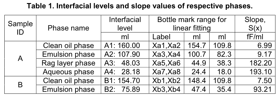
It is noted that for chemical ranking, slope value, S(x), derived from capacitance value can be directly used without converting it to water content using a calibration curve because they correlate monotonically and share the same trend. The higher the slope value the higher water content in the corresponding phase, such as (1) water content in the clean oil phase is higher in bottle B than in bottle A due to that slope value is higher for the respective phase in bottle B (7.50 fF/ml) than in bottle A (6.99 fF/ml); (2) water content in the emulsion phase is significantly higher in bottle B than in bottle A due to that slope value is higher for the respective phase in bottle B (93.21 fF/ml) than in bottle A (9.17 fF/ml); and (3) water content increases from the clean oil phase through the aqueous phase in bottle A due to that slope values are in ascending order: 6.99, 9.17, 182.20 and 193.10 fF/ml. This is a very unique feature of this technique in chemical screening tests.
It is also noted that derivative C'(x) has the same meaning as the slope value S(x) if the bottle mark x range is narrow enough for linear fitting. Hence, C'(x) curves can be directly used for chemical ranking in a chemical screening test, excluding those spikes for phase boundary identification.
A spike of the derivative C'(x) represents an additional capacitance of the respective interface, which is a measure of excess charges, Q, at the interface and can be evaluated using the area of the spike or be calculated directly using capacitance change over the spike,
Q = C(x2) – C(x1) (5),
where x1 and x2 are the onset and offset of the spike. In other words, interfacial thickness, ![]() , can also be evaluated by
, can also be evaluated by
![]() = x2 – x1————————(6).
= x2 – x1————————(6).
Sample A’s rag layer/aqueous (A4) interfacial thickness ![]() is 7.09 ml (= 31.64 ml – 24.55 ml) and sample B’s clean oil/emulsion (B2) interfacial thickness
is 7.09 ml (= 31.64 ml – 24.55 ml) and sample B’s clean oil/emulsion (B2) interfacial thickness ![]() is 8.19 ml (= 80.24 ml – 72.05 ml), they can be further converted to actual thicknesses of 2.73 mm and 3.15 mm respectively using its bottle mark factor (0.3841 mm/ml). Interfacial thickness can be used as an additional marker for evaluating chemical performance, the greater the interfacial thickness the harder for oil/water phase separation.
is 8.19 ml (= 80.24 ml – 72.05 ml), they can be further converted to actual thicknesses of 2.73 mm and 3.15 mm respectively using its bottle mark factor (0.3841 mm/ml). Interfacial thickness can be used as an additional marker for evaluating chemical performance, the greater the interfacial thickness the harder for oil/water phase separation.
5. Aqueous phase quality analysis
The scanned curves can also be used for qualitative analysis of oil in the respective bottom aqueous phase. Capacitance is sensitive to salt content in water when the salt content is below 1%, capacitance becomes insensitive when the salt content is higher than 1%. Salt content in water is higher than 1% in almost all field situations. In a batch of samples, salt content in water can be close to each other. Hence, the scanned curves can be used for qualitative analysis of oil in the respective bottom aqueous phase. The higher the derivative value the better the aqueous phase quality or the less the oil content in the aqueous phase. For example, it can be observed in Fig.7 that Ca'(x) is higher than Cb'(x) when the bottle mark x is below the rag/aqueous interfacial level A4, meaning aqueous phase quality in bottle A was better than that in bottle B, which was still an emulsion.
6. Surface/interfacial tension measurement
Both surface and interfacial tensions can be measured accurately using the MCSWA instrument directly or using a more compact form of the instrument, namely multi-channel tensiometer, wherein technical detail is provided.